
Welcome to the fourth installment of the Get Connected blog series here on Analog Wire! In my previous post we explored jitter from a high level examining random jitter (RJ) and the components of deterministic jitter (DJ) that all come together to make up total jitter (TJ). In this post, we will discuss lab techniques to measure RJ and the components of DJ accurately.
Measuring jitter properly can be quite a daunting task, but if you understand the definitions of each component that we covered in Get Connected: Jitter then your measurement is meaningful and comprehensible. We learned that RJ is unbounded and probabilistic which makes it very hard to put a max value on. Because of this, RJ is typically specified as an RMS value instead of a peak-to-peak value. Since RJ is an RMS value, the measurement is most accurately taken in the frequency domain using a phase noise analyzer (PNA) because a PNA will have a lower noise floor than an oscilloscope. The PNA is also better for this measurement because it allows you to see at what frequency(s) the problematic spurs occur. The PNA’s noise floor is extremely important because if the noise floor of your DUT is lower than the PNA noise floor, your measurement results will be skewed towards the PNA and not the DUT. This is known better around the lab as measuring the equipment.
The PNA self-detects the carrier frequency of the incoming signal and measures the RMS jitter value of the signal by integrating over the limits that are selected. Setting the integration limits on the PNA to start at 1kHz and stop at 100MHz away from the carrier is not unheard of but a typical integration would stop at 40MHz away from the carrier frequency as most of the RMS jitter has already been captured. Check out an example of an additive jitter measurement that I performed on the SN65LVELT22 LVTTL to LVPECL translator in Figure 1. The additive RMS jitter at 2GHz was measured to be approximately 91.41fs RMS.
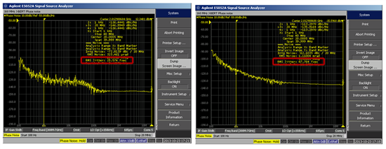
Figure 1

This is not the only approach to making an RMS jitter measurement as it can also be done in the time domain using a histogram and implementing a Gaussian tail-fitting model. The PNA method will give us the best, or closest, measurement of our actual RMS jitter value as it has a lower noise floor than an oscilloscope.
DJ is a bit different as it is a bounded quantity which is measured as peak-to-peak value on a digital oscilloscope. When doing DJ measurements in my lab I typically use a real time digital oscilloscope with at least five times the bandwidth of the signal that I am trying to measure. If the scope does not possess enough bandwidth it will not capture enough of the signals harmonics and the digital signal will start to look like a sine wave. This ultimately shows up in your measurement as excessive DJ and renders your measurement invalid. The other important piece of the puzzle when measuring DJ is reliable software that performs the jitter decomposition. The math involved with jitter decomposition is very cumbersome which is why the most convenient way to measure DJ is through a software package and not by hand. Most of the newer model oscilloscopes have a jitter software package that you can buy in addition to your scope.
With the measured RJ value from the PNA and the jitter decomposition software we can now dissect the DJ into its components and measure the TJ reliably. A technique that the Agilent DCA-X oscilloscope allows you to do is fix the RJ number while doing a jitter measurement. This is useful since RJ is unbounded and continues to rise in time, which in turn makes the TJ number rise as well. Figure 2 below shows the Agilent DCA-X jitter GUI and the components that it calculates. In these two screen shots I measure a case with no ISI and some ISI using a KR signal. The RJ was not fixed in this instance but the scope calculates out the TJ, PJ (pk-pk & RMS), ISI, and DCD for us. The DCA-X also generates several histograms showing the standard deviation and a BER Jitter Bathtub curve that a confidence level for a certain BER can be extrapolated from.

Figure 2
For more information on application specific solutions like the SN65LVET22 LVTTL to LVPECL translator, please visit the High Speed Interface Forum in TI’s E2E™ Community and check out existing posts from engineers already using TI interface products, or create a new thread to address your specific application.
Please join me for my next post in the Get Connected series where we will take a deep dive into the MLVDS standard and an application specific example. If you are not connected you can get connected with one of the broadest Interface portfolio’s in the industry.
Leave your comments in the section below if you’d like to hear more about anything mentioned in this post or if there is a topic you'd like to see us tackle in the future!
And be sure to check out the full Get Connected series!